
The DC response of a simple common-emitter amplifier
In tutorial 2, we obtained the ideal BJT parameters of the 2N2222A transistor. We can now use this transistor to build more complex circuits like amplifiers. Let us start with a simple common emitter amplifier, shown below:
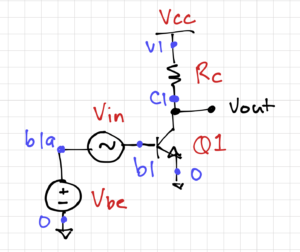
The SPICE netlist is given below. Let’s save this as ‘amplifier_ce.sp‘.
1 2 3 4 5 6 7 8 9 10 11 12 13 14 15 16 17 18 19 20 21 22 23 | * Common Emitter Amplifiers* LPA 2020-04-18.include 2N2222A.lib.options savecurrentsQ1 c1 b1 0 Q2n2222aRc v1 c1 2.5kVcc v1 0 dc 5Vin b1 b1a dc 0 sin(0 10m 1k)Vbe b1a 0 dc 682.73m.controldc Vin -100m 100m 1mwrdata ce_amp_transfer_sim.dat v(c1) @Q1[ic]tran 1u 5mwrdata ce_amp_transient_sim.dat v(b1) v(c1) .endc.end |
If we want to bias the transistor at a collector current of 1mA, we can use our results in the previous tutorials, and set  . Recall that by writing a KVL equation at the output:

Thus, for  and
and  , we need a resistor
  to give us a
  . Note that choosing
  , we maximize the output swing of the amplifier.
Also note that the total base voltage is:

Vbe + Vin
Let’s look at the first analysis in the control portion of the netlist: the DC analysis. By sweeping Vin, we are merely sweeping the value of the base voltage 100mV below 682.73mV (582.73mV) to 100mV above it (782.73mV).
Thus, if we start sweeping Vin, we should see an exponential increase in  , and an exponential decrease in
  , and hence the output voltage:

Let’s use the following Python script to run the simulation, and plot the amplifier output voltage and the BJT’s collector current:
1 2 3 4 5 6 7 8 9 10 11 12 13 14 15 16 17 18 19 20 21 22 23 24 25 26 27 28 29 30 31 32 33 34 35 36 37 38 39 40 41 42 43 44 45 46 47 48 49 50 51 52 53 54 55 56 57 58 59 60 61 62 63 64 65 66 67 68 69 70 71 | import matplotlib.pyplot as pltimport numpy as npimport eee51, g51 # load constantsg51.init_global_constants()# run ngspicecfg = { 'spice' : '/Applications/ngspice/bin/ngspice', 'cir_dir' : '/Users/louis/Documents/UPEEEI/Classes/EEE 51/Mini Projects/', 'cir_file' : 'amplifier_ce.sp', 'transfer_data' : 'ce_amp_transfer_sim.dat' }# note: you can do this from the command line and just process the data files# this was done here for convenienceeee51.run_spice(cfg)# open the transfer characteristics data file and get the datavin = [] # declare list for vinvout = [] # declare a list for voutic = [] # declare a list for icwith open(cfg['transfer_data'], 'r') as f: for line in f: vin.append(float(line.split()[0])) vout.append(float(line.split()[1])) ic.append(float(line.split()[3])) bjt_n = 1.2610858394025979reqd_vbe = 682.73e-3Rc = 2.5e3g51.update_bjt_VA(-15.550605626760145) index, vin_sim = eee51.find_in_data(vin, 0.0)vo_dc = vout[index]# define the plot parametersplt_cfg = { 'grid_linestyle' : 'dotted', 'title' : r'Common Emitter Amplifier DC Transfer Curve', 'xlabel' : r'$v_{in}$ [mV]', 'ylabel' : r'$v_{out}$ [V]', 'legend_loc' : 'upper left', 'add_legend' : True, 'legend_title' : None }# plot the amplifier transfer characteristicsfig = plt.figure()ax = fig.add_subplot(1, 1, 1)ax.plot(eee51.scale_vec(vin, g51.milli), vout, '--', \ label = r'$v_{OUT}$ with $R_C=$2.5 k$\Omega$')ax2 = ax.twinx()ax2.set_ylabel(r'$I_C$ [mA]')ax2.plot(eee51.scale_vec(vin, g51.milli), eee51.scale_vec(ic, g51.milli), \ ':', color='orangered', label = r'$I_C$')ax2.legend(loc='upper right')eee51.add_vline_text(ax, 0, 0, r'$V_{BE}$ = ' + \ '{:.1f}mV'.format(reqd_vbe/g51.milli))eee51.add_hline_text(ax, vo_dc, -75, \ r'$V_{OUT}=$' + '{:.2f}V'.format(vo_dc))eee51.label_plot(plt_cfg, fig, ax)plt.savefig('2N2222A_ce_transfer.png') |
This produces the following graph:
As expected, and  are exponential. Also, note that the current saturates to just below 2mA, again as expected, since
  .
.

We do incur a small error. Since our output voltage is 2.58V instead of 2.5V. This means that our collector current is slightly lower than 1mA. The significance of this error will depend on the application where this amplifier will be used. The key idea here is that we know exactly how to adjust  if we really need to be very accurate.
From amplifier transfer characteristic in Figure 1, we can see that a small change in the input voltage produces a large change in the output. Thus, we can estimate the small signal gain of the amplifier as:

Given the ideal BJT parameters, we can also estimate the gain of the amplifier using small signal analysis:


Thus:

Numerically calculating the derivative of the transfer function, and using the small signal parameters to estimate the gain:
73 74 75 76 77 78 79 80 81 82 83 84 85 86 87 88 89 90 91 92 93 94 95 96 97 98 99 100 101 102 103 104 105 106 107 108 109 110 | # get the gain via the slope of the transfer curvegain_ss = np.diff(vout)/np.diff(vin)ro_calc = abs(g51.bjt_VA) / ic[index] gm_calc = ic[index]/(bjt_n * g51.VT)gain_calc = -gm_calc * eee51.r_parallel([Rc, ro_calc])# define the plot parametersplt_cfg = { 'grid_linestyle' : 'dotted', 'title' : r'Common Emitter Amplifier Small Signal Gain', 'xlabel' : r'$v_{in}$ [mV]', 'ylabel' : r'Gain $A_v = \frac{\partial v_{out}}{\partial v_{in}}$', 'legend_loc' : 'upper left', 'add_legend' : True, 'legend_title' : None }# plot the amplifier transfer characteristicsfig = plt.figure()ax = fig.add_subplot(1, 1, 1)ax.plot(eee51.scale_vec(vin[1:], g51.milli), gain_ss, '--', \ label = r'$v_{OUT}$ with $R_C=$2.5 k$\Omega$')eee51.add_vline_text(ax, 0, -50, r'$V_{BE}$ = ' + \ '{:.1f}mV'.format(reqd_vbe/g51.milli))eee51.add_hline_text(ax, gain_ss[index-1], -75, \ r'$A_v=${:.2f}V'.format(gain_ss[index-1]))ax.text(-100, -100, r'$g_m =\frac{I_C}{n\cdot V_T}=$' + \ '{:.2f} mS'.format(gm_calc/g51.milli))ax.text(-100, -110, r'$a_v=-g_m \cdot (R_c||r_o)=${:.2f}'.format(gain_calc))eee51.label_plot(plt_cfg, fig, ax)plt.savefig('2N2222A_ce_gain.png') |
We then get the following results:
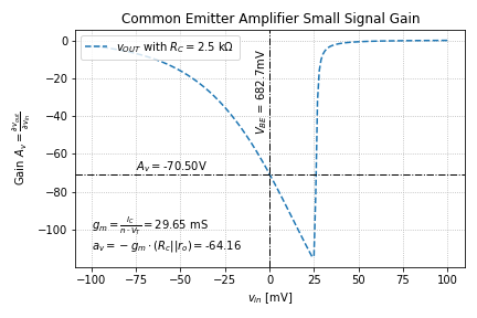
There is a very good agreement between the simulated gain and the gain predicted by our ideal BJT models. Notice that the gain is not constant, and depends on the value of the input voltage, but the variation is small if the inputs are “small”.
It is important to note that since our hand analysis uses relatively simple models, we do not expect the resulting values to be exactly the same as our simulation results. In fact, we can get as much as 20% errors in some cases. This is normal. Again, the crucial concept here is that we understand the relationships between the various parameters, such that we can adjust our design and/or analysis accordingly.
End of Tutorial 3
Congratulations! You have just plotted the DC transfer characteristics of a simple common emitter amplifier and obtained its small signal gain.