
BJT Small Signal Parameters
So far in tutorial 2, we have obtained the transistor parameters:
- The Early Voltage,
 (tutorial 2A)
 - Saturation current,
 (tutorial 2B)
 - Ideality factor or emission coefficient of the base-emitter junction,
 (tutorial 2B)
 - The forward current gain,
 (tutorial 2C)
Having these parameters will enable us to calculate the small signal equivalent circuit of the BJT.
Transistor Transconductance
We can obtain the transistor transconductance from the transistor transfer characteristics:

We will once again use the netlist below as circuit3.sp, and again, we are going to use the data file ‘bjt_transfer_sim.dat‘.
1 2 3 4 5 6 7 8 9 10 11 12 13 14 15 16 17 18 19 20 21 22 23 24 | * Transistor Characteristic Curves* LPA 2020-04-16.include 2N2222A.lib.options savecurrentsQ1 c1 b1 0 Q2n2222aVbe b1 0 dc 0Vce c1 0 dc 0.2Q2 c2 b1 0 Q2n2222aVce2 c2 0 dc 2.5.controldc Vbe 500m 750m 1mwrdata bjt_transfer_sim.dat @Q1[ic] @Q2[ic] @Q2[ib]dc Vce 30m 5 10m Vbe 0.65 0.7 0.01wrdata bjt_output_sim.dat @Q1[ic] .endc.end |
Let’s use the following Python script to run the simulation, read the results, and plot the transfer characteristics of the BJT.
1 2 3 4 5 6 7 8 9 10 11 12 13 14 15 16 17 18 19 20 21 22 23 24 25 26 27 28 29 30 31 32 33 34 35 36 37 38 39 40 41 42 43 44 45 46 47 48 49 50 51 52 53 54 55 56 57 58 59 60 61 62 63 64 65 66 67 68 69 70 71 72 73 74 75 76 77 78 79 80 81 82 83 84 85 86 87 88 89 90 | import matplotlib.pyplot as pltimport numpy as npfrom si_prefix import si_formatimport eee51, g51 # load constantsg51.init_global_constants()specs = { 'ic' : 1e-3, 'vce' : 2.5 } # run ngspicecfg = { 'spice' : '/Applications/ngspice/bin/ngspice', 'cir_dir' : '/Users/louis/Documents/UPEEEI/Classes/EEE 51/Mini Projects/', 'cir_file' : 'circuit3.sp', 'transfer_data' : 'bjt_transfer_sim.dat', 'output_data' : 'bjt_output_sim.dat' }# note: you can do this from the command line and just process the data files# this was done here for convenienceeee51.run_spice(cfg)# open the transfer characteristics data file and get the datavbe = [] # declare list for vbeic = [] # declare a list for ic with vce = vce,sat = 0.2Vic2 = [] # declare a list for ic with vce = 2.5Vib2 = [] # declare a list for ib with vce = 2.5V with open(cfg['transfer_data'], 'r') as f: for line in f: vbe.append(float(line.split()[0])) ic.append(float(line.split()[1])) ic2.append(float(line.split()[3])) ib2.append(float(line.split()[5]))# convert to mV and mAic_mA = eee51.scale_vec(ic, g51.milli)vbe_mV = eee51.scale_vec(vbe, g51.milli)bjt_beta = [a/b for a, b in zip(ic2, ib2)]# bjt parameters from our dc characterizationbjt_Is = 6.924988420125876e-13bjt_n = 1.2610858394025979g51.update_bjt_VA(-15.550605626760145) g51.update_bjt_vce(specs['vce']) # calculate the vbe needed for vce = 2.5Vreqd_vbe = eee51.bjt_find_vbe(specs['ic'], specs['vce'], \ bjt_Is, bjt_n, g51.bjt_VA)# generate the ic for the ideal bjt model # using our values for Is, n, and VA at vce = 2.5Vic_ideal = [eee51.ideal_bjt_transfer(v, bjt_Is, bjt_n) for v in vbe]ic_ideal_mA = eee51.scale_vec(ic_ideal, g51.milli)# define the plot parametersplt_cfg = { 'grid_linestyle' : 'dotted', 'title' : 'BJT 2N2222A Transfer Characteristics', 'xlabel' : r'$V_{BE}$ [V]', 'ylabel' : r'$I_C$ [mA]', 'legend_loc' : 'upper left', 'add_legend' : True, 'legend_title' : None }# plot the transfer characteristics at 2.5Vfig = plt.figure()ax = fig.add_subplot(1, 1, 1)ax.plot(vbe_mV, eee51.scale_vec(ic2, g51.milli), '--', \ label = 'simulation ($V_{CE}$=2.5V)')ax.plot(vbe_mV, ic_ideal_mA, \ label = 'ideal BJT using $I_S$=' + \ si_format(bjt_Is, precision=2) + r'A, $n$={:.2f}, and '.format(bjt_n) + \ r'$|V_A|$={:.2f}'.format(abs(g51.bjt_VA)))eee51.add_vline_text(ax, reqd_vbe/g51.milli, 2.5, '$V_{BE}$ = ' + \ '{:.1f}mV'.format(reqd_vbe/g51.milli))eee51.add_hline_text(ax, specs['ic']/g51.milli, 550, \ '$I_C$ = {:.1f}mA'.format(specs['ic']/g51.milli))eee51.label_plot(plt_cfg, fig, ax) |
We then take the derivative of the transfer function, as well as calculate the transconductance from the ideal BJT equation:

Note that we can already calculate the remaining small signal parameters from the BJT parameters we have obtained:


92 93 94 95 96 97 98 99 100 101 102 103 104 105 106 107 108 109 110 111 112 113 114 115 116 117 118 119 120 121 122 123 124 125 126 127 128 129 130 131 132 133 134 135 136 137 138 139 140 141 142 143 144 145 146 147 148 149 150 151 | # get the derivative of ic with respect to vbedic2 = np.diff(ic2)/np.diff(vbe)dic_ideal = np.diff(ic_ideal)/np.diff(vbe)index, vbe_sim = eee51.find_in_data(vbe, reqd_vbe)gm_sim = dic2[index-1]gm_ideal = dic_ideal[index-1]# calculate the bjt small signal parametersgm_calc = ic2[index]/(bjt_n * g51.VT)ro_calc = abs(g51.bjt_VA) / ic2[index] rpi_calc = bjt_beta[index] / gm_calcao_calc = gm_calc * ro_calc# define the plot parametersplt_cfg = { 'grid_linestyle' : 'dotted', 'title' : r'BJT 2N2222A ${\partial I_C}/{\partial V_{BE}}$', 'xlabel' : r'$V_{BE}$ [V]', 'ylabel' : r'${\partial I_C}/{\partial V_{BE}}$ [mS]', 'legend_loc' : 'upper left', 'add_legend' : True, 'legend_title' : None }# plot the derivative of transfer characteristics at 2.5Vfig = plt.figure()ax = fig.add_subplot(1, 1, 1)ax.plot(vbe_mV[1:], eee51.scale_vec(dic2, g51.milli), '--', \ label = 'simulation ($V_{CE}$=2.5V)')ax.plot(vbe_mV[1:], eee51.scale_vec(dic_ideal, g51.milli), \ label = 'ideal BJT using $I_S$=' + \ si_format(bjt_Is, precision=2) + r'A, $n$={:.2f}, and '.format(bjt_n) + \ r'$|V_A|$={:.2f}V'.format(abs(g51.bjt_VA)))eee51.add_vline_text(ax, reqd_vbe/g51.milli, 75, r'$V_{BE}$ = ' + \ '{:.1f}mV'.format(reqd_vbe/g51.milli))eee51.add_hline_text(ax, gm_sim/g51.milli, 600, \ r'$g_m$ = {:.2f}mS (sim)'.format(gm_sim/g51.milli))ax.text(500, 175, r'$|V_A|$={:.2f}V, '.format(abs(g51.bjt_VA)) + \ r'$\beta_{DC}=$' + '{:.2f}'.format(bjt_beta[index]) )ax.text(500, 150, r'$g_{m,ideal}$' + '={:.2f} mS'.format(gm_ideal/g51.milli))ax.text(500, 125, r'$g_m=\frac{I_C}{n \cdot V_T}=$' + \ '{:.2f} mS'.format(gm_calc/g51.milli))ax.text(500, 100, r'$r_o=\frac{|V_A|}{I_C}=$' + \ si_format(ro_calc, precision=2) + '$\Omega$')ax.text(580, 100, r'$r_\pi=\frac{\beta_{DC}}{g_m}=$' + \ si_format(rpi_calc, precision=2) + '$\Omega$')ax.text(500, 75, r'$a_o=|g_m \cdot r_o|=${:.2f}'.format(ao_calc))eee51.label_plot(plt_cfg, fig, ax)plt.savefig('2N2222A_small_signal_2500mV.png') |
We end up with the small signal parameters of the 2N2222A for  and
and  :
:
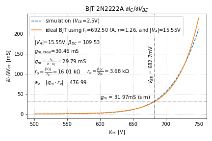
Notice that the difference between the simulation data and the ideal BJT model is much more pronounced. Since the small signal parameters depend on the derivatives of the transistor characteristics, the matching between the first derivatives must also be taken into account.
It is very important to remember that the small signal BJT parameters change with the bias current.
End of Tutorial 2D
Congratulations! You have just derived the BJT small signal model parameters from the transistor characteristics.