EEE 51 Tutorial 2A

BJT Output Characteristics: Finding $V_A$

In tutorial 1, we simulated the behavior of $I_C$ as we vary the $V_{BE}$ of a 2N2222A NPN transistor, and we plotted this using ngspice. However, if we want to use this transistor in designing more complex circuits, or if we want to analyze circuits using this BJT, we would need to extract useful information from the simulation results.

In tutorial 2, we will obtain the transistor parameters:

The Early Voltage, $V_A$ (tutorial 2A)
Saturation current, $I_S$ (tutorial 2B)
Ideality factor or emission coefficient of the base-emitter junction, $n$ (tutorial 2B)
The forward current gain, $\beta_{DC}$ (tutorial 2C)

Having these parameters will enable us to estimate the collector current:

$I_C=I_S \cdot e^{\frac{V_{BE}}{n \cdot V_T}}\cdot \left(1+\frac{V_{CE}}{\left|V_A\right|}\right)$

Where $V_T=\frac{k \cdot T}{q}$ is the thermal voltage, or the voltage equivalent of temperature.

Transistor Output Characteristics

In order to get the Early Voltage, we need to determine the transistor output characteristics. We will use the netlist below as circuit2.sp:

* Transistor Characteristic Curves
* LPA 2020-04-16

.include 2N2222A.lib
.options savecurrents

Q1		c1 b1 0		Q2n2222a
Vbe		b1 0		dc 0
Vce		c1 0 		dc 0.2

.control

dc Vbe 500m 750m 1m
wrdata bjt_transfer_sim.dat @Q1[ic]

dc Vce 30m 5 10m Vbe 0.65 0.7 0.01
wrdata bjt_output_sim.dat @Q1[ic]
 
.endc

.end

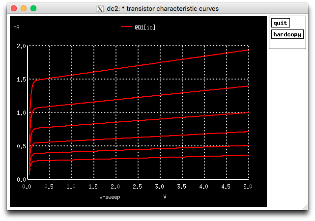
Notice that we added another DC sweep (at line 16) that is a bit different from the DC sweep we ran in tutorial 1 (line 13). This DC sweep is a nested DC sweep, where we are sweeping two variables:

First, Vce is swept from 30mV to 5V in 10mV steps starting with a Vbe of 0.65V,
Then Vbe is increased by 0.01V, and Vce swept once again from 30mV to 5V. This repeats until a Vbe of 0.7 is reached.

The nested DC analysis allows us to create families of curves. And once again, we write the transistor current data to a file named ‘bjt_output_sim.dat‘ using the wrdata command.

Running ngspice and loading the netlist:

******
** ngspice-31 : Circuit level simulation program
** The U. C. Berkeley CAD Group
** Copyright 1985-1994, Regents of the University of California.
** Please get your ngspice manual from http://ngspice.sourceforge.net/docs.html
** Please file your bug-reports at http://ngspice.sourceforge.net/bugrep.html
******
ngspice 1 -> source circuit2.sp

Circuit: * transistor characteristic curves

Doing analysis at TEMP = 27.000000 and TNOM = 27.000000


No. of Data Rows : 251
Doing analysis at TEMP = 27.000000 and TNOM = 27.000000


No. of Data Rows : 2988
ngspice 2 -> plot @Q1[ic]
ngspice 3 ->

Note that both DC analyses were run. Running the plot @Q1[ic] command plots the results of the last analysis, and gives us the graph below:

Figure 1: The BJT output characteristics.

Obtaining the Early Voltage

We can automate this process by using ngspice in batch mode, i.e. running the simulator from the command line, and reading the output file using Python, and do the processing automatically.

You can run the simulation at the command line using: ngspice circuit2.sp.
One very good environment for Python3 is Spyder. You can download this for multiple platforms, and the easiest way to install Spyder is as part of the Anaconda distribution, also available for various operating systems.

Below is a simple Python script for running ngspice, reading its output, and finding the Early Voltage from the output characteristics of the BJT. It depends on two other Python files, (eee51.py and g51.py), that contain convenient functions and constants.

First, we import Python modules that contain computing and plotting functions:

#!/usr/bin/env python3
# -*- coding: utf-8 -*-
"""
Created on Sun Apr 19 15:15:35 2020

@author: louis
"""

import matplotlib.pyplot as plt
from scipy.optimize import curve_fit
import numpy as np
import math
from statistics import mean

Then we load our custom modules (eee51.py and g51.py), that contain convenient functions and constants specific to EEE 51. Note that all functions and variables that start with eee51.xxx and g51.xxx are defined in these custom modules.

import eee51, g51 

# load constants and global variables, referenced by g51.*
g51.init_global_constants()

Before running ngspice, we need to provide the filenames and locations of the netlist and the output files. You need to change this part to run the script on your system.

# run ngspice
cfg = {
        'spice' : '/Applications/ngspice/bin/ngspice', 
        'cir_dir' : '/Users/louis/Documents/UPEEEI/Classes/EEE 51/Mini Projects/',
        'cir_file' : 'circuit2.sp',
        'transfer_data' : 'bjt_transfer_sim.dat',
        'output_data' : 'bjt_output_sim.dat'
        }

# note: you can do this from the command line and just process the data files
# this was done here for convenience
eee51.run_spice(cfg)

After running the simulation, we read in the output characteristics data from the output file and load them into Python lists.

# open the output characteristics data file and get the data
vbe = np.linspace(0.65, 0.7, 6, endpoint=True)     # from the simulation setup
vce = []    # declare an empty list to store vce data
ic = [[] for v in range(len(vbe))]  # declare a 2d array to store the currents
                                    # for the different values of vbe

# read the data file
# you can open the data file produced by ngspice and examine the file format
m = 0
with open(cfg['output_data'], 'r') as f:
    for i, line in enumerate(f):
        
        if i == 0:
            vswp0 = float(line.split()[0])
        
        vswp = float(line.split()[0])
        
        if i != 0 and vswp == vswp0:
            m += 1

        if m == 0:
            vce.append(vswp)
            
        ic[m].append(float(line.split()[1]))

Once we have all the data loaded into lists, we can use the curve_fit function to fit lines over the linear parts of the curve (e.g. when 1V $\leq V_{CE} \leq$ 4V) and extrapolate it to their respective x-intercepts.

# fit the data to the ideal BJT out characteristic and find the Early Voltage (VA)
# fit the line over the linear range of the curves 
# e.g. from 1V to 4V
ind1, vce1 = eee51.find_in_data(vce, 1)
ind4, vce4 = eee51.find_in_data(vce, 4) 

line_m = []     # declare an array of 'slopes'
line_b = []     # declare an array of 'y-intercepts'
line_VA = []    # declare an array of 'x-intercepts' or in this case, VA

# use curve_fit to get the slopes and y-intercepts then caculate VA
for j, v in enumerate(vbe):
    popt, pcov = curve_fit(eee51.line_eq, vce[ind1:ind4], ic[j][ind1:ind4])
    line_m.append(popt[0])
    line_b.append(popt[1])
    line_VA.append(-popt[1]/popt[0])

# declare the x values for plotting the curve-fitted lines
line_x = np.linspace(math.floor(min(line_VA)), max(vce), 100)
g51.update_bjt_VA(mean(line_VA))     
# use the mean value of VA
# yay! we got an estimate for VA

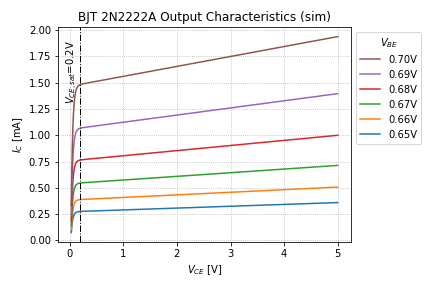
We then plot the output characteristics and save it to an image file, shown in Figure 2.

# define the plot parameters
plt_cfg = {
        'grid_linestyle' : 'dotted',
        'title' : 'BJT 2N2222A Output Characteristics (sim)',
        'xlabel' : r'$V_{CE}$ [V]',
        'ylabel' : r'$I_C$ [mA]',
        'legend_loc' : 'upper left',
        'add_legend' : False
        }

# plot the output characteristics
fig = plt.figure()
ax = fig.add_subplot(1, 1, 1)

for m, v in enumerate(vbe):
    ax.plot(vce, eee51.scale_vec(ic[m], g51.milli), \
        label = '{:.2f}V'.format(v))

eee51.add_vline_text(ax, 0.2, 1.3, r'$V_{CE,sat}$=' + '{:.1f}V'.format(0.2))

# reorder the legend entries for easier reading
handles, labels = ax.get_legend_handles_labels()
ax.legend(handles[::-1], labels[::-1], title='$V_{BE}$', bbox_to_anchor=(1, 1))

eee51.label_plot(plt_cfg, fig, ax)
plt.savefig('2N2222A_output.png')

Figure 2: The 2N2222A BJT output characteristics plotted using Python. Note that the saturation voltage, as expected, is around 200mV.

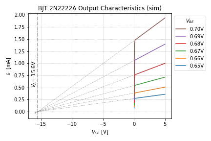
We then plot the output characteristics with the extrapolated curve-fitted lines and their x-intercepts, to get the Early Voltage, $V_A$ . Again, the plot is saved as an image and is shown in Figure 3.

# plot the output characteristics and curve-fitted lines to show VA
fig = plt.figure()
ax = fig.add_subplot(1, 1, 1)

for m, v in enumerate(vbe):
    ax.plot(vce, eee51.scale_vec(ic[m], g51.milli), \
        label = '{:.2f}V'.format(v))

# plot the curve-fitted lines
for m, b in zip(line_m, line_b):
    ax.plot(line_x, eee51.scale_vec(eee51.line_eq(line_x, m, b), g51.milli), \
        '-.', color='gray', linewidth='0.5')

eee51.add_vline_text(ax, g51.bjt_VA, 0.5, r'$V_A$={:.1f}V'.format(g51.bjt_VA))

# reorder the legend entries for easier reading
handles, labels = ax.get_legend_handles_labels()
ax.legend(handles[::-1], labels[::-1], title='$V_{BE}$', bbox_to_anchor=(1, 1))
eee51.label_plot(plt_cfg, fig, ax)
plt.savefig('2N2222A_output_VA.png')

Figure 3: The extrapolated lines for calculating the Early Voltage.

Thus, for this transistor, the Early Voltage, $V_A\approx -15.6\mathrm{V}$ .

Note that this method is very convenient, since we can get a good approximation of the Early Voltage even without knowing the other BJT parameters.

End of Tutorial 2A

Congratulations! You have successfully performed a nested DC sweep in ngspice and processed the output characteristics of the BJT to get its Early Voltage.