BJT Transfer Characteristics: Finding  and
and 
In tutorial 1, we simulated the behavior of ![]() as we vary the
as we vary the ![]() of a 2N2222A NPN transistor, and we plotted this using ngspice. However, if we want to use this transistor in designing more complex circuits, or if we want to analyze circuits using this BJT, we would need to extract useful information from the simulation results.
of a 2N2222A NPN transistor, and we plotted this using ngspice. However, if we want to use this transistor in designing more complex circuits, or if we want to analyze circuits using this BJT, we would need to extract useful information from the simulation results.
In tutorial 2, we will obtain the transistor parameters:
- The Early Voltage,
 (tutorial 2A)
 - Saturation current,
 (tutorial 2B)
 - Ideality factor or emission coefficient of the base-emitter junction,
 (tutorial 2B)
 - The forward current gain,
 (tutorial 2C)
Having these parameters will enable us to estimate the collector current:
![]()
Where ![]() is the thermal voltage, or the voltage equivalent of temperature.
is the thermal voltage, or the voltage equivalent of temperature.
Transistor Transfer Characteristics
In order to get the BJT transfer characteristics, we will use the netlist below as circuit3.sp, but this time, we are going to use the data file ‘bjt_transfer_sim.dat‘.
* Transistor Characteristic Curves
* LPA 2020-04-16

.include 2N2222A.lib
.options savecurrents

Q1		c1 b1 0		Q2n2222a
Vbe		b1 0		dc 0
Vce		c1 0 		dc 0.2

Q2		c2 b1 0		Q2n2222a
Vce2		c2 0 		dc 2.5

.control

dc Vbe 500m 750m 1m
wrdata bjt_transfer_sim.dat @Q1[ic] @Q2[ic] @Q2[ib]

dc Vce 30m 5 10m Vbe 0.65 0.7 0.01
wrdata bjt_output_sim.dat @Q1[ic]

.endc

.end
Note that we instantiated two transistors, Q1 and Q2. The base of the transistors are connected to Vbe, but the transistors have different voltage sources at their collector terminals: Vce for Q1, and Vce2 for Q2. This way, we can simulate what happens if we use two different ![]() values (0.2V and 2.5V) at the same time, instead of one after the other.
values (0.2V and 2.5V) at the same time, instead of one after the other.
Let’s also try and figure out the ![]() we need to generate a collector current of 1mA,
we need to generate a collector current of 1mA,
We will use the following Python script to run ngspice, and read in the simulation data. You might need to install the si_prefix package by running
conda install -c sci-bots si-prefix
import matplotlib.pyplot as plt
from scipy.optimize import curve_fit
from si_prefix import si_format
import eee51, g51

# load constants and global variables, referenced by g51.*
g51.init_global_constants()

specs = {
        'ic' : 1e-3,
        'vce' : 2.5
        }

# run ngspice
cfg = {
        'spice' : '/Applications/ngspice/bin/ngspice',
        'cir_dir' : '/Users/louis/Documents/UPEEEI/Classes/EEE 51/Mini Projects/',
        'cir_file' : 'circuit3.sp',
        'transfer_data' : 'bjt_transfer_sim.dat',
        'output_data' : 'bjt_output_sim.dat'
        }

# note: you can do this from the command line and just process the data files
# this was done here for convenience
eee51.run_spice(cfg)

# to get the rest of the BJT parameters, let's use the transfer characteristics
# open the transfer characteristics data file and get the data
vbe = []    # declare list for vbe
ic = []     # declare a list for ic with vce = vce,sat = 0.2V
ic2 = []    # declare a list for ic with vce = 2.5V
            # we'll use this to check our model
ib2 = []    # declare a list for the base currents at vce = 2.5V

with open(cfg['transfer_data'], 'r') as f:
    for line in f:
        vbe.append(float(line.split()[0]))
        ic.append(float(line.split()[1]))
        ic2.append(float(line.split()[3]))
        ib2.append(float(line.split()[5]))

# convert to mV and mA
ic_mA = eee51.scale_vec(ic, g51.milli)
vbe_mV = eee51.scale_vec(vbe, g51.milli)

# fit the data to the ideal BJT transfer characteristic and find Is
# fit using the data at vce = 0.2V
g51.update_bjt_vce(0.2)

# use VA from our previous analysis
g51.update_bjt_VA(-15.550605626760145)
We can then run the curve_fit function once again, but this time, instead of fitting to a line, we will fit the data to the ideal BJT equation:
![]()
popt, pcov = curve_fit(eee51.ideal_bjt_transfer, vbe, ic)
bjt_Is = popt[0]    # yay! we get an estimate for Is and n
bjt_n = popt[1]
Now that we know ![]() ,
, ![]() , and
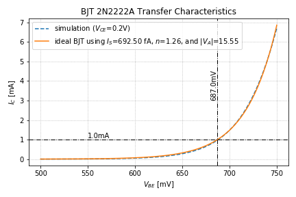
, and ![]() , we can use this to model our transistor. Let’s compare our model with the simulation results and plot the comparison, as shown in Figure 1.
, we can use this to model our transistor. Let’s compare our model with the simulation results and plot the comparison, as shown in Figure 1.
# generate the ic for the ideal bjt model
# using our values for Is, n, and VA at vce = 0.2V
ic_ideal = [eee51.ideal_bjt_transfer(v, bjt_Is, bjt_n) for v in vbe]
ic_ideal_mA = eee51.scale_vec(ic_ideal, g51.milli)

# get the value of vbe that will result in a 1mA ic using the simulation results
index_spec_sim, ic_spec_sim = eee51.find_in_data(ic, specs['ic'])
vbe_spec_sim = vbe[index_spec_sim]
vbe_spec_sim_mV = vbe_spec_sim/g51.milli

# get the value of vbe that will result in a 1mA ic using the our model
index_spec_ideal, ic_spec_ideal = eee51.find_in_data(ic_ideal, specs['ic'])
vbe_spec_ideal = vbe[index_spec_ideal]
vbe_spec_ideal_mV = vbe_spec_ideal/g51.milli

plt_cfg = {
        'grid_linestyle' : 'dotted',
        'title' : 'BJT 2N2222A Transfer Characteristics',
        'xlabel' : r'$V_{BE}$ [mV]',
        'ylabel' : r'$I_C$ [mA]',
        'legend_loc' : 'upper left',
        'add_legend' : True,
        'legend_title' : None
        }

# plot the transfer characteristics at 200mV
fig = plt.figure()
ax = fig.add_subplot(1, 1, 1)
ax.plot(vbe_mV, ic_mA, '--', label = 'simulation ($V_{CE}$=0.2V)')
ax.plot(vbe_mV, ic_ideal_mA, \
    label = 'ideal BJT using $I_S$=' + \
    si_format(bjt_Is, precision=2) + r'A, $n$={:.2f}, and '.format(bjt_n) + \
    r'$|V_A|$={:.2f}'.format(abs(g51.bjt_VA)))

# add_vline_text(ax, vbe_1mA_sim_mV, 3, '{:.1f}mV'.format(vbe_1mA_sim_mV))
eee51.add_vline_text(ax, vbe_spec_ideal_mV, 3, '{:.1f}mV'.format(vbe_spec_ideal_mV))

eee51.add_hline_text(ax, specs['ic']/g51.milli, 550, \
    '{:.1f}mA'.format(specs['ic']/g51.milli))

eee51.label_plot(plt_cfg, fig, ax)
plt.savefig('2N2222A_transfer_200mV.png')

 and the required
  to generate a collector current of 1mA.
As we can see, our model using the ideal BJT equation agrees well with the simulation data at ![]() .
.
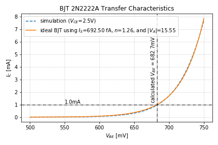
Let’s plot the transfer characteristics, but now, let’s use the simulation data for ![]() . The comparison plot is shown in Figure 2.
. The comparison plot is shown in Figure 2.
# calculate the vbe needed for vce = 2.5V
reqd_vbe = eee51.bjt_find_vbe(specs['ic'], specs['vce'], \
    bjt_Is, bjt_n, g51.bjt_VA)

# generate the ic for the ideal bjt model
# using our values for Is, n, and VA at vce = 2.5V

g51.update_bjt_vce(specs['vce'])

ic_ideal = [eee51.ideal_bjt_transfer(v, bjt_Is, bjt_n) for v in vbe]
ic_ideal_mA = eee51.scale_vec(ic_ideal, g51.milli)

# plot the transfer characteristics at 2.5V
fig = plt.figure()
ax = fig.add_subplot(1, 1, 1)
ax.plot(vbe_mV, eee51.scale_vec(ic2, g51.milli), '--', \
    label = 'simulation ($V_{CE}$=2.5V)')
ax.plot(vbe_mV, ic_ideal_mA, \
    label = 'ideal BJT using $I_S$=' + \
    si_format(bjt_Is, precision=2) + r'A, $n$={:.2f}, and '.format(bjt_n) + \
    r'$|V_A|$={:.2f}'.format(abs(g51.bjt_VA)))

eee51.add_vline_text(ax, reqd_vbe/g51.milli, 1.1, 'calculated $V_{BE}$ = ' + \
    '{:.1f}mV'.format(reqd_vbe/g51.milli))

eee51.add_hline_text(ax, specs['ic']/g51.milli, 550, \
    '{:.1f}mA'.format(specs['ic']/g51.milli))

eee51.label_plot(plt_cfg, fig, ax)
plt.savefig('2N2222A_transfer_2500mV.png')

 and the required
  to generate a collector current of 1mA.
We can see that our model using the ideal BJT equation also agrees well with the simulation data at ![]() .
.
Given our values for ![]() ,
, ![]() , and
, and ![]() , we can now use our ideal BJT equation to predict the DC behavior of the collector current,
, we can now use our ideal BJT equation to predict the DC behavior of the collector current, ![]() .
.
End of Tutorial 2B
Congratulations! You have successfully derived the saturation current and the ideality factor of the 2N2222A NPN transistor from the BJT’s transfer characteristics.
