BJT Input Characteristics: Finding 
In tutorial 1, we simulated the behavior of ![]() as we vary the
as we vary the ![]() of a 2N2222A NPN transistor, and we plotted this using ngspice. However, if we want to use this transistor in designing more complex circuits, or if we want to analyze circuits using this BJT, we would need to extract useful information from the simulation results.
of a 2N2222A NPN transistor, and we plotted this using ngspice. However, if we want to use this transistor in designing more complex circuits, or if we want to analyze circuits using this BJT, we would need to extract useful information from the simulation results.
In tutorial 2, we will obtain the transistor parameters:
- The Early Voltage,
 (tutorial 2A)
 - Saturation current,
 (tutorial 2B)
 - Ideality factor or emission coefficient of the base-emitter junction,
 (tutorial 2B)
 - The forward current gain,
 (tutorial 2C)
Having these parameters will enable us to estimate the collector current:
![]()
Where ![]() is the thermal voltage, or the voltage equivalent of temperature.
is the thermal voltage, or the voltage equivalent of temperature.
Additionally, we would also like a way to estimate the base current from the collector current.
Transistor Input Characteristics
We will use the netlist below as circuit3.sp, and again, we are going to use the data file ‘bjt_transfer_sim.dat‘.
* Transistor Characteristic Curves
* LPA 2020-04-16

.include 2N2222A.lib
.options savecurrents

Q1		c1 b1 0		Q2n2222a
Vbe		b1 0		dc 0
Vce		c1 0 		dc 0.2

Q2		c2 b1 0		Q2n2222a
Vce2		c2 0 		dc 2.5

.control

dc Vbe 500m 750m 1m
wrdata bjt_transfer_sim.dat @Q1[ic] @Q2[ic] @Q2[ib]

dc Vce 30m 5 10m Vbe 0.65 0.7 0.01
wrdata bjt_output_sim.dat @Q1[ic]

.endc

.end
Notice that we have already saved the base current data of transistor Q2 to the file ‘bjt_transfer_sim.dat‘. Recall that transistor Q2 is the transistor with ![]() .
.
We will use the following Python script to run ngspice, and read in the simulation data. As we have done before, we will run ngspice, then load the data into Python as lists. We also add in the BJT parameters we have obtained so far.
import matplotlib.pyplot as plt
import eee51, g51

# load constants and global variables, referenced by g51.*
g51.init_global_constants()

specs = {
        'ic' : 1e-3,
        'vce' : 2.5
        }

# run ngspice
cfg = {
        'spice' : '/Applications/ngspice/bin/ngspice',
        'cir_dir' : '/Users/louis/Documents/UPEEEI/Classes/EEE 51/Mini Projects/',
        'cir_file' : 'circuit3.sp',
        'transfer_data' : 'bjt_transfer_sim.dat',
        'output_data' : 'bjt_output_sim.dat'
        }

# note: you can do this from the command line and just process the data files
# this was done here for convenience
eee51.run_spice(cfg)

# to get the rest of the BJT parameters, let's use the transfer characteristics
# open the transfer characteristics data file and get the data
vbe = []    # declare list for vbe
ic2 = []    # declare a list for ic with vce = 2.5V
            # we'll use this to check our model
ib2 = []    # declare a list for the base currents at vce = 2.5V

with open(cfg['transfer_data'], 'r') as f:
    for line in f:
        vbe.append(float(line.split()[0]))
        ic2.append(float(line.split()[3]))
        ib2.append(float(line.split()[5]))

# convert to mV
vbe_mV = eee51.scale_vec(vbe, g51.milli)

# plot the transistor dc beta
g51.update_bjt_VA(-15.550605626760145)
bjt_n = 1.2610858394025979
bjt_Is = 6.924988420125876e-13
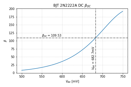
We then calculate and plot the ratio of the collector current to the base current.
# calculate the vbe needed for vce = 2.5V
reqd_vbe = eee51.bjt_find_vbe(specs['ic'], specs['vce'], \
    bjt_Is, bjt_n, g51.bjt_VA)

bjt_beta = [a/b for a, b in zip(ic2, ib2)]

index, vbe_sim = eee51.find_in_data(vbe, reqd_vbe)

plt_cfg = {
        'grid_linestyle' : 'dotted',
        'title' : r'BJT 2N2222A DC $\beta_{DC}$',
        'xlabel' : r'$V_{BE}$ [mV]',
        'ylabel' : r'$\beta$',
        'legend_loc' : 'upper left',
        'add_legend' : False,
        'legend_title' : None
        }

fig = plt.figure()
ax = fig.add_subplot(1, 1, 1)
ax.plot(vbe_mV, bjt_beta, \
    label = 'simulation ($V_{CE}$=2.5V)')

eee51.add_vline_text(ax, reqd_vbe/g51.milli, 10, '$V_{BE}$ = ' + \
    '{:.1f}mV'.format(reqd_vbe/g51.milli))

eee51.add_hline_text(ax, bjt_beta[index], 550, \
    r'$\beta_{DC}=$' + '{:.2f}'.format(bjt_beta[index]))

eee51.label_plot(plt_cfg, fig, ax)
plt.savefig('2N2222A_beta_dc.png')
We then get the plot in Figure 1.

 as a function of
In tutorial 2, we have seen that, for the 2N2222A NPN transistor, we can use the ideal BJT equations with the following parameters:
End of Tutorial 2C
Congratulations! You have successfully derived the ideal BJT parameters for the 2N2222A BJT from its simulated input, output, and transfer characteristics.
