The transient response of a simple common-emitter amplifier
In tutorial 3, we explored the DC transfer characteristics of our simple common emitter amplifier, and derived its small signal gain. In this tutorial, we will look at how the amplifier responds to small signal time-varying inputs.
We will again use the SPICE netlist ‘amplifier_ce.sp‘.
* Common Emitter Amplifiers
* LPA 2020-04-18

.include 2N2222A.lib
.options savecurrents

Q1		c1 b1 0	Q2n2222a
Rc	 	v1 c1	2.5k
Vcc		v1 0	dc 5
Vin		b1 b1a	dc 0 sin(0 10m 1k)
Vbe		b1a 0	dc 682.73m

.control

dc Vin -100m 100m 1m
wrdata ce_amp_transfer_sim.dat v(c1) @Q1[ic]

tran 1u 5m
wrdata ce_amp_transient_sim.dat v(b1) v(c1)

.endc

.end
We will use the output file from the transient analysis, second analysis in the control block.
A transient analysis is called using the tran command, with the format
tran <step time> <stop time>
The analysis calculates the behavior of the circuit, updated every <step_time>, until the <stop time>. In this case, we run the simulation for 5ms, updating the values every 1![]() s. Also notice that the
s. Also notice that the Vin voltage source, aside from the dc 0 term, has a time-varying term: sin(0 10m 1k). This specifies that during the transient analysis, Vin is a sinusoidal source, with 0V DC offset, 10mV amplitude, and a frequency of 1kHz.
We will use the Python script below to run the simulation and read in the data:
import matplotlib.pyplot as plt
import numpy as np
import eee51, g51

# load constants
g51.init_global_constants()

# run ngspice
cfg = {
        'spice' : '/Applications/ngspice/bin/ngspice',
        'cir_dir' : '/Users/louis/Documents/UPEEEI/Classes/EEE 51/Mini Projects/',
        'cir_file' : 'amplifier_ce.sp',
        'transient_data' : 'ce_amp_transient_sim.dat'
        }

# note: you can do this from the command line and just process the data files
# this was done here for convenience
eee51.run_spice(cfg)

# open the transfer characteristics data file and get the data
t = []   # declare list for the time variable
vin = []    # declare list for vin
vout = []   # declare a list for vout

with open(cfg['transient_data'], 'r') as f:
    for line in f:
        t.append(float(line.split()[0]))
        vin.append(float(line.split()[1]))
        vout.append(float(line.split()[3]))

vinpp = max(vin) - min(vin)
voutpp = max(vout) - min(vout)

# define the plot parameters
plt_cfg = {
        'grid_linestyle' : 'dotted',
        'title' : r'Common Emitter Amplifier DC Transient Response',
        'xlabel' : r'Time [ms]',
        'ylabel' : r'Voltage [V]',
        'legend_loc' : 'upper left',
        'add_legend' : True,
        'legend_title' : None
        }

# plot the amplifier transfer characteristics
fig = plt.figure()
ax = fig.add_subplot(1, 1, 1)

ax.plot(eee51.scale_vec(t, g51.milli), vin, '-', \
    label = r'$v_{IN}$ = ' + '{:.2f} '.format(vinpp/g51.milli) + r'$mV_{p-p}$')

ax.plot(eee51.scale_vec(t, g51.milli), vout, '-', \
    label = r'$v_{OUT}$ = ' + '{:.2f} '.format(voutpp) + r'$V_{p-p}$')

ax.set_ylim(0, 5)

eee51.add_hline_text(ax, 682.7e-3, 0, \
    r'$V_{IN}=$' + '{:.2f}mV'.format(682.7))

eee51.add_hline_text(ax, 2.58, 0, \
    r'$V_{OUT}=$' + '{:.2f}V'.format(2.58))

ax.text(3.1, 4.5, r'$a_v=\frac{V_{OUT,p-p}}{V_{IN,p-p}}=$' + \
    '{:.2f}'.format(voutpp/vinpp))

eee51.label_plot(plt_cfg, fig, ax)
plt.savefig('2N2222A_ce_transient.png')
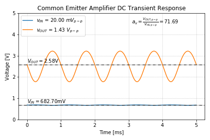
We then get the following plot:

It is important to note that at the input of the amplifier, the sinusoid is superimposed on the input DC voltage of 682.7mV, and the output voltage sinusoid is superimposed on the output DC voltage of 2.58V.
If we take the ratio of the peak-to-peak output voltage to the peak-to-peak input voltage, we see that the magnitude of the gain is 71.69, which agrees with our hand analysis in tutorial 3.
The plot in Figure 1 is very hard to read since the input voltage is relatively small compared to the output voltage. We can add another axis to Python plot the input voltage to examine the phase of the output relative to the input.
# define the plot parameters
plt_cfg = {
        'grid_linestyle' : 'dotted',
        'title' : r'Common Emitter Amplifier DC Transient Response',
        'xlabel' : r'Time [ms]',
        'ylabel' : r'$V_{OUT}$ [V]',
        'legend_loc' : 'upper left',
        'add_legend' : True,
        'legend_title' : None
        }

# plot the amplifier transfer characteristics
fig = plt.figure()
ax = fig.add_subplot(1, 1, 1)
ax2 = ax.twinx()

ax2.plot(eee51.scale_vec(t, g51.milli), eee51.scale_vec(vin, g51.milli), '-', \
    label = r'$v_{IN}$ = ' + '{:.2f} '.format(vinpp/g51.milli) + r'$mV_{p-p}$')

ax.plot(eee51.scale_vec(t, g51.milli), vout, '-', color = 'orangered', \
    label = r'$v_{OUT}$ = ' + '{:.2f} '.format(voutpp) + r'$V_{p-p}$')

ax2.set_ylabel(r'$V_{IN}$ [mV]')
ax2.legend(loc='upper right')

ax.set_ylim(0, 5)
ax2.set_ylim(650, 900)


eee51.add_hline_text(ax2, 682.7, 3.75, \
    r'$V_{IN}=$' + '{:.2f}mV'.format(682.7))

eee51.add_hline_text(ax, 2.58, 0, \
    r'$V_{OUT}=$' + '{:.2f}V'.format(2.58))

ax.text(0, 4, r'$a_v=\frac{V_{OUT,p-p}}{V_{IN,p-p}}=$' + \
    '{:.2f}'.format(voutpp/vinpp))

eee51.label_plot(plt_cfg, fig, ax)
plt.savefig('2N2222A_ce_transient_zoom.png')
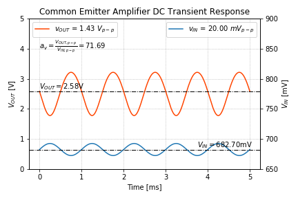
This results in the following plot:

Now the input voltage y-axis is on the right, and the output voltage y-axis is on the left. Notice the different y-axis scales.
We can then verify that the amplifier is an “inverting” amplifier, where the output decreases when the input increases. This should be expected, since as the input voltage increases, the BJT collector current increases, increasing the voltage across Rc, thus pushing the output voltage down.
We recall from tutorial 3 that the gain is not constant over the range of the input. This causes “distortion” at the output, and is a characteristic of all semiconductor electronic amplifiers.
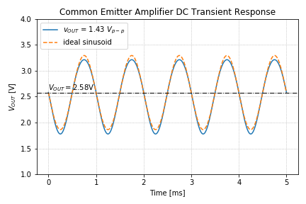
Distortion is defined as the deviation of a voltage signal from an ideal sinusoid, and even though this is a fundamental property of all semiconductor amplifiers, there are many circuit techniques that can reduce this distortion to suit a specific application. For us, it is important to understand that distortion exists, and that the output voltage is not a perfect sinusoid.
Let us plot the output voltage and compare it to an ideal sinusoid:
# ideal sinusoid
am = 1.43/2
w = 2 * np.pi * 1e3
ideal_sin = [-am * np.sin(w * tx) + 2.58 for tx in t]

# define the plot parameters
plt_cfg = {
        'grid_linestyle' : 'dotted',
        'title' : r'Common Emitter Amplifier DC Transient Response',
        'xlabel' : r'Time [ms]',
        'ylabel' : r'$V_{OUT}$ [V]',
        'legend_loc' : 'upper left',
        'add_legend' : True,
        'legend_title' : None
        }

# plot the amplifier transfer characteristics
fig = plt.figure()
ax = fig.add_subplot(1, 1, 1)


ax.plot(eee51.scale_vec(t, g51.milli), vout, '-', \
    label = r'$v_{OUT}$ = ' + '{:.2f} '.format(voutpp) + r'$V_{p-p}$')

ax.plot(eee51.scale_vec(t, g51.milli), ideal_sin, '--', \
    label = r'ideal sinusoid')

ax.set_ylim(1, 4)

eee51.add_hline_text(ax, 2.58, 0, \
    r'$V_{OUT}=$' + '{:.2f}V'.format(2.58))

eee51.label_plot(plt_cfg, fig, ax)
plt.savefig('2N2222A_ce_transient_output_disto.png')
Our code generates the following graph:

From Figure 3, we can see the difference between an ideal sinusoid and the output voltage. Note that, as expected, there is more gain at the negative peaks compared to the positive peaks as seen in Figure 3 of tutorial 3.
End of Tutorial 4
Congratulations! You just ran a SPICE transient analysis, and examined the input and output voltage waveforms of the common emitter amplifier.
